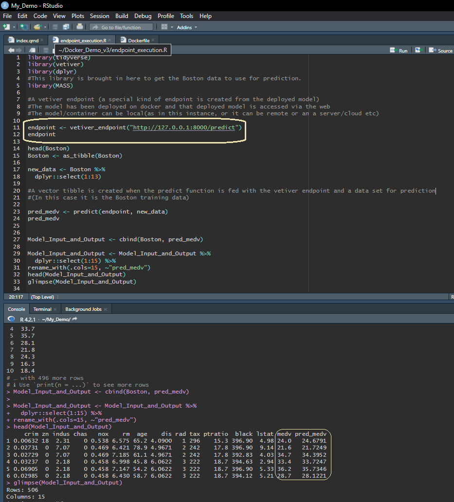
Containerizing R Models for Scaling & Production

Author

Akila Balas

Published

Oct 5, 2023

Preface

In many scenarios an analyst would prototype a model in their favorite language, say in R or Python. Insights from the model results and its empirical applications would evince interest in the need for periodic delivery of the insights. Of course, one could use Markdown/or Quarto documents to automate and send the insights to business leaders on a periodic basis right from your local computer. But there are many scenarios when the need for ‘self-help’ insights are sought and hence scaling and automation would be vital . But at this stage the analyst would find themselves handing it off. This would result in frustration, low morale and endless hours of trying to re-invent the wheels in another language and ensure the model delivers the same precision and quality as the original prototype.

This need not be the case.

A step by step approach to developing and serving web APIs(Plumber APIs) and scaling your prototype and containerizing them on Docker will be shared along with three illustrations and hope that you as the reader would benefit from them.

This document will predominantly discuss and showcase the scaling and containerizing of models developed in the R programming language(which has an abundance of libraries spanning statistical and machine learning methods) with some references/pointers to containerize python based models as well.

Scaling models through hosting APIs can be performed on various platforms. A brief discussion on some of the options will be given during the overview of Web APIs.

In this paper, the emphasis will be on scaling an application through containerization. The process of packaging all the software code and the operating system with just the necessary libraries and dependencies to run an application is containerization.

Docker(2023) is an open platform for containerizing your applications. One can build and run docker containers on your local laptops, Virtual Machines or on the cloud. You could develop the application locally and the Docker containers can be easily portable from one environment to the other; an image created in one environment can be shared to other environments through Docker Hub. One often hears the terms Docker images and containers. An image is a read-only template for creating a container. And a container is a runnable instance of the image.

Your dockerfile is akin to a recipe that provides instructions to Docker to develop a customized container that meets your needs. When you run the image built from the dockerfile, an instance of a container is created - which is an isolated software environment that is ready to execute your application. An in-depth overview of Docker is available on the link shared above.

You can install the Docker Desktop on your local machine by visiting the Docker site using the following link - Docker Desktop Installation Guide.

Podman is another containerizing option that is gaining popularity momentum and deems a quick introduction.
As defined in the Podman Project website - Podman is a daemonless, open source, Linux native tool designed to make it easy to find, run, build, share and deploy applications using Open Containers Initiative Containers and Container Images.” It is worth reading the details on this option so you are well aware of and prepared to leverage the same where necessary.

The Rocker Project- provides high-quality Docker images containing R environments with the provision of base R images that can be mirrored from the project and portable to spin up a base environment in Docker to containerize your R application. You can choose from several options which can vary based on the version of R you would like to mirror and or any pre-configured libraries that are built-in etc., including building shiny applications at scale.
(Please refer to the following blog for intrinsic details on containerizing and Scaling Shiny Applications.)

All Rocker images are based on the Debian Linux distribution.

The above link to the Rocker Project site and the following additional article on Introduction to Rocker(2017) provide a depth of details and intricacies.

For the illustrations and demos shown here, Docker images and containers will be created on a Local Machine/Desktop along with pointers on portability to the cloud and any additional platform specific details (specific to Google Cloud).

Serving the Model - (Illustrations)

Three examples detailing the serving of a prediction model via a web API will be illustrated.

The tool used in these illustrations is predominantly RStudio (with VS Code in some instances); one can also use Jupyter Notebook on a local machine(or Vertex AI), or on Google Colab(hosted Jupyter Notebook using your Google account) based on one’s preferences. Versatility is a boon.

Illustration I

Random Forest Model and Plumber API (on Local Machine)

The Boston Housing data found in the MASS library is used for all three illustrations. This data set (containing information collected from the US Census service) has 506 cases/instances and 14 attributes (13 predictor variables & the dependent variable Median Housing value-medv).

The intricacies of building a Random Forest model, fine-tuning etc will not be discussed. The emphasis will be on developing the Web API and subsequent containerization.

A specific folder will be used for each illustration and all applicable files used and generated for the illustration will be stored there for ease of serving the model as a Web API on the local machine as well as for subsequent containerization on Docker and the serving of the Web API and prediction through Docker.

library(MASS)
library(randomForest)
library(dplyr)
library(yaml)
glimpse(Boston)
1
MASS library is called for importing the Boston Housing data.
Rows: 506
Columns: 14
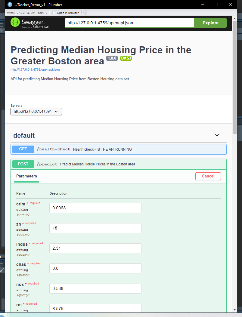
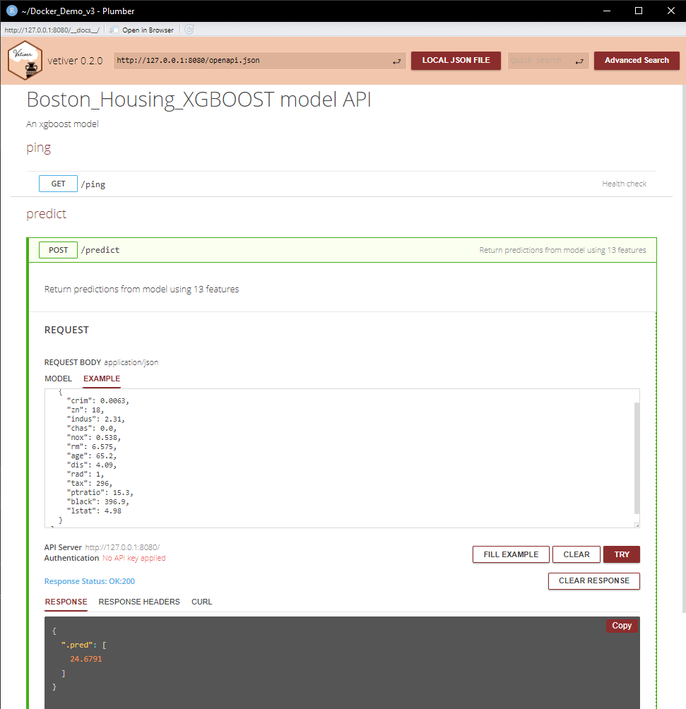
$ crim    <dbl> 0.00632, 0.02731, 0.02729, 0.03237, 0.06905, 0.02985, 0.08829,…
$ zn      <dbl> 18.0, 0.0, 0.0, 0.0, 0.0, 0.0, 12.5, 12.5, 12.5, 12.5, 12.5, 1…
$ indus   <dbl> 2.31, 7.07, 7.07, 2.18, 2.18, 2.18, 7.87, 7.87, 7.87, 7.87, 7.…
$ chas    <int> 0, 0, 0, 0, 0, 0, 0, 0, 0, 0, 0, 0, 0, 0, 0, 0, 0, 0, 0, 0, 0,…
$ nox     <dbl> 0.538, 0.469, 0.469, 0.458, 0.458, 0.458, 0.524, 0.524, 0.524,…
$ rm      <dbl> 6.575, 6.421, 7.185, 6.998, 7.147, 6.430, 6.012, 6.172, 5.631,…
$ age     <dbl> 65.2, 78.9, 61.1, 45.8, 54.2, 58.7, 66.6, 96.1, 100.0, 85.9, 9…
$ dis     <dbl> 4.0900, 4.9671, 4.9671, 6.0622, 6.0622, 6.0622, 5.5605, 5.9505…
$ rad     <int> 1, 2, 2, 3, 3, 3, 5, 5, 5, 5, 5, 5, 5, 4, 4, 4, 4, 4, 4, 4, 4,…
$ tax     <dbl> 296, 242, 242, 222, 222, 222, 311, 311, 311, 311, 311, 311, 31…
$ ptratio <dbl> 15.3, 17.8, 17.8, 18.7, 18.7, 18.7, 15.2, 15.2, 15.2, 15.2, 15…
$ black   <dbl> 396.90, 396.90, 392.83, 394.63, 396.90, 394.12, 395.60, 396.90…
$ lstat   <dbl> 4.98, 9.14, 4.03, 2.94, 5.33, 5.21, 12.43, 19.15, 29.93, 17.10…
$ medv    <dbl> 24.0, 21.6, 34.7, 33.4, 36.2, 28.7, 22.9, 27.1, 16.5, 18.9, 15…

Greater details on the above attributes can be found within the MASS library/package as well as on several public & academic sites.

A random forest model is run for Illustration I.

## Build a Random Forest Model
boston_rf_v1 <- randomForest(medv ~., data = Boston, mtry =3, ntree = 500, importance = TRUE)

The model is saved in the same project/folder that contains all files relevant to Illustration I.

## save the model
saveRDS(boston_rf_v1, "boston_rf_v1.rds")

Having built our Random Forest Model and saved it in the Project folder, we will next develop an API that can accept inputs for prediction. In the case of the Boston Housing Market data - one can supply new data with unique values for 13 predictor variables and the predicted housing price will be generated through a Web API (- a Plumber API in the R programming world).

What is a Plumber API

The Plumber Library allows you to create web API by adding/incorporating special comments/annotations to your existing R code. These special comments make the R code available as API endpoints that is available on the web.

The following links provide greater details on the workings of the Plumber Library as well as a series of articles on deploying Plumber APIs.

Additionally, the CRAN documentation details can be found in Plumber Library on CRAN where one can find greater details on fine-tuning your Plumber R Code and the API to fit your needs.

Below we are building a plumber file that will generate the API when executed. The #* are plumber annotations that precede variables and or a specific action they perform - such as #* get, #* predict etc.

In the below illustration we first read in the model we built earlier. In this plumber file we have two endpoints:
–@get /health-check which does a system check that our API is working.
–@post /predict which calls the model and predicts the Median Housing price on the new data. They also accept parameters as evident from the code.

One can easily decipher the other plumber annotations in the below Plumber file

The saved Random Forest model is passed to this plumber file. The Plumber API developed below can now be hosted on a local machine for illustration.

## Plumber.R file (Illustration I)

library(plumber)
library(randomForest)

boston_rf_v1 <- readRDS("boston_rf_v1.rds")

#* Health check - IS THE API RUNNING
#* @get /health-check

status <- function() {
  list(
    message = "Hello There! All is well!",
    time = Sys.time()
  )
}

#* @apiTitle Predicting Median Housing Price in the Greater Boston area
#* @apiDescription API for predicting Median Housing Price from Boston Housing data 
#* @param crim
#* @param zn
#* @param indus
#* @param chas
#* @param nox
#* @param rm
#* @param age
#* @param dis
#* @param rad
#* @param tax
#* @param ptratio
#* @param black
#* @param lstat

#* Predict Median House Prices in the Boston area

#* @post /predict

Medv <- function(crim, zn, indus, chas, nox, rm, age, dis, rad, tax, ptratio, black, lstat) 
  {
  crim <- as.numeric(crim)
  zn <- as.numeric(zn)
 indus <- as.numeric(indus)
 chas <- as.numeric(chas)
 nox <- as.numeric(nox)
 rm <- as.numeric(rm)
 age <- as.numeric(age)
 dis <- as.numeric(dis)
 rad <- as.numeric(rad)
 tax <- as.numeric(tax)
 ptraio <- as.numeric(ptratio)
 black <- as.numeric(black)
 lstat <- as.numeric(lstat) 
  
     new_data <- data.frame(crim = as.numeric(crim),
                        zn = as.numeric(zn),
                        indus = as.numeric(indus),
                        chas = as.numeric(chas),
                        nox = as.numeric(nox),
                        rm = as.numeric(rm),
                        age = as.numeric(age),
                        dis = as.numeric(dis),
                        rad = as.numeric(rad),
                        tax = as.numeric(tax),
                        ptratio = as.numeric(ptratio),
                        black = as.numeric(black),
                        lstat = as.numeric(lstat)
                       )

  predict(boston_rf_v1, new_data)
}

The above plumber.R code is also saved in our project folder as shown in Figure 1.

The plumber API can be hosted by clicking the ‘RunAPI’ button within R studio or can be ‘plumbed’ from console or notebook.

Figure 1 - (Illustration I - List of Files)

Figure 1: Version 1 Model - List of files for API Generation

The swagger UI is automatically generated when you run the Plumber API. The swagger UI or Postman UI can also be used independently to harness additional features to test, upload json files etc.

The swagger output from running the Plumber-API is shown below.

Th first screen has two buttons - the –@GET button and the –@POST button. (a) Swagger

The –@get is to ensure that the API is error-free and for system check.

The –@post is the vital one here as this serves us the prediction values for the Random Forest Model. Here we have 13 independent variables - and we can enter the values we would like a prediction on into each of those distinct parameter boxes. The response body shows the predicted value for the inputted parameter values. (Swagger (b) & (c) shown below)

Figure 2 - The swagger outputs that are observed when the Plumber API is launched

(a) Swagger
(b) Swagger
(c) Swagger
Figure 2: Swagger Output from running Plumber API

The plumber file in this illustration used the arduous approach of naming every variable used in the predict function and also requires the stipulation that each variable is in the appropriate format(i.e. numeric etc ).

In Illustration II the approach will be more streamlined by creating a function that calls the incoming HTTP requests and the outgoing HTTP response. Additionally, the API specification YAML file pre-populates swagger UI with example values and also helps helps pre-define the parameter formats.

The Plumber API in this illustration was hosted on a local machine. One cannot serve Incoming requests from a local machine for a myriad of reasons ranging from the dynamic nature of your local machine’s IP address, feasibility of handling multiple requests and security to name a few.

There are a variety of options that one can consider to scale and host plumber APIs.

  • Posit Connect is a publishing platform from Posit(formerly RStudio) where you can host your API with push button options and which automatically manages dependencies.

  • DigitalOcean (a cloud computing provider). They offer a simple to spin up of a Linux Virtual Machine and one can choose the bandwidth used based on one’s needs. The following plumber companion package plumberDeploy gives more info on using DigitalOcean to deploy Plumber APIs.

  • Docker - A platform built on Linux Containers that provides an isolated environment. A more detailed introduction was shared in the introductory preface because Illustration II & III in this document will showcase the hosting of Plumber APIs on Docker using custom images and containers specific to the illustrations.

Illustration II

A Random Forest Model Hosted on Docker with a customized Open-API file

In this illustration, we continue to use the same data-set - Boston Housing data and the same Random Forest model as in the previous illustration. But the Plumber API will be hosted on Docker.

Docker Desktop was installed on the local machine and ‘up and running’ before any Docker related commands were executed in the terminal.

## Build a Random Forest Model
boston_rf_v2 <- randomForest(medv ~., data = Boston, mtry =3, ntree = 500, importance = TRUE)
## save the model
saveRDS(boston_rf_v2, "boston_rf_v2.rds")

In addition to hosting the Plumber API through Docker, what is different in this illustration is that the Plumber file is generated in a less arduous way - by utilizing a function that captures the incoming HTTP request and the outgoing HTTP response - without having to enumerate each parameter and specifying their format etc. Additionally, an open API Yaml file is used to pre-define the format of the parameters as well as pre-populate the swagger UI. These changes make the UI easier to use and interact with.

## Plumber.R file (Illustration II)

library(plumber)
library(randomForest)
library(yaml)

boston_rf_v2 <- readRDS("boston_rf_v2.rds")

#* Health check - IS THE API RUNNING
#* @get /health-check

status <- function() {
  list(
    status = "Hello There! All is well!",
    time = Sys.time()
  )
}

# @apiTitle - This Will be pulled from YAML file 
# @apiDescription This will also be pulled from the YAML file

#* Predict Median House Prices in the Boston area

#* @post /predict

#* @serializer json

## Note the function is given a name (f1) for the sake of smooth code execution for html prep, but is not needed 
## when actually executing the plumber API in the console/editor/notebook

f1 <- function(req, res)
{
  predict(boston_rf_v2, newdata = as.data.frame(req$body))
}

## The Yaml file is provided for api spec so the swagger json file will be pre-populated with an example and 
## the parameters will be pre-formatted.

#* @plumber 
 f2 <- function(pr)
  {
    pr %>%
      pr_set_api_spec(yaml::read_yaml("boston_openapi.yaml"))
 }
Tip
  • In Illustrations I & II - the Swagger UI is shown/utilized (as the default UI)
  • You have the option to specify the UI/API Visualizer(Swagger, RapiDoc or Redoc) by incorporating the specifics in your plumber API code.
  • Explore the layouts of the other UIs /API visualizers; (RapiDoc has cool features and a user-friendly layout!)
    Note: The Redoc API visualizer does not provide the ‘Try/Execute’ button unless the security schemes are configured.*
  • The pr_set_doc function can be used to specify/customize the UI.

The below visual Figure 3 - shows the list of files in the current project/directory and includes the Open API Yaml file that is called into the Plumber API code.

Additionally, a snapshot showing the format of the Open API is shown below in Figure 4.

Figure 3 - (Illustration II - List of Files )

Figure 3: Version 2 Model - List of files for API Generation

Figure 4 - Open API File (Format)

Figure 4: Open API - Yaml file - Boston Housing Data

Since this Illustration will be dockerized - a Dockerfile is created and placed in the same project folder as the other files that would be used in the building of the API. Docker will be able to find the necessary files if they are in the directory where Docker build commands are executed.

Dockerfile Essentials - Figure 5
  • The dockerfile is built from the base image of R version 4.2.1 since that is the version on the Local Machine on which the illustration was built.
  • Essential Linux libraries along with essential R libraries to be installed in the container are shown.
  • The Random forest model object, the plumber file (with the plumbing instructions) and the open api yaml files are copied into the dockerfile to instruct docker to do the same onto the containers for API execution and hosting.
  • The final line provides instruction to use the R Plumber file to deploy the API on the local portal of choice.

Figure 5 - Dockerfile - Illustration II

Figure 5: Dockerfile (Model2) - For building the Docker Image

The following visuals show the execution of Docker Commands for building the image and creating the container. As can be noted from the terminal, the current working directory is changed to reflect the path in which all the relevant files are located for building the image and container.

Figure 6 - Docker Commands on PowerShell terminal - Random Forest

Powershell Terminal
Figure 6: Docker Commands for building Images & Containers(Terminal)

The Docker Image and Container for the Random Forest Model Illustration are created by the execution of the above Docker commands and are shown below. When one clicks the container that is active/running - it takes you to the endpoint - the API where the model is being served.

Figure 7 - Docker desktop highlighting image & container for the Random Forest Model .

(a) Docker Image Random Forest
(b) Docker Container Random Forest
Figure 7: Docker Image & Container generated from DockerFile

There are two endpoints that are available as evident in the Swagger UI. One is the -GET endpoint which ensures that our API is working and the other is -POST endpoint that will serve the Predicted Median Housing Price for a given set of input values for the parameters. The HTTP connection is available to serve the response.

One can execute/try out the API with the pre-populated example in the UI and receive the predicted value as a response. Additional json data can also be incorporated into the example and executed.

Please note that even though the files are on the local machine, and the Docker container is on the Local Desktop - the Plumber APi and endpoint can be accessed from anywhere remote using the endpoint URL and the response/predictions can be served.

Figure 8 - Swagger Output from running Plumber API on the Docker

(a) Swagger UI System Check
(b) Swagger UI System Check
Figure 8: Swagger Output from running Plumber API - System Health Check - Boston_rf_v2 Docker Container
(a) Swagger-Model Prediction Example
(b) Swagger-Model Prediction Example
Figure 9: Swagger Output from Plumber API on Docker Container - Predicting Housing Price -Example Illustration - Boston_rf_v2

To further illustrate this - a new R session is opened - it can be any remote session while the container with our model is running on Docker and feed a sample data set to the endpoint.

In the illustration below in Figure 10, the endpoint is being fed with a data source to generate multiple predictions. A sample of the Boston Housing training data-set is passed to the endpoint as a json file and the predicted median housing price is then merged with the original data set to showcase the comparison of the actual and predicted values along with the various parameters.

Figure 10 - Endpoint Illustration with multiple predictions from a data source

(a) Endpoint Illustration- Random Forest
(b) Endpoint Illustration - Random Forest
Figure 10: Endpoint Illustration - JSON output and data-frame output of predicted values - Random Forest

Illustration III

An XGBoost - Vetiver Model

This illustration will also be the using the same Boston Housing data (from the MASS library) that was also used in Illustrations I & II.

As with the Random Forest model used in Illustrations I & II, details regarding the intricacies of the model and parameter fine-tuning etc will not be discussed.

The model in this illustration will be (1) an XGBoost model and (2) it will also be a vetiver model, built on the vetiver library which would enable the auto-generation of files for scaling/deploying the model as well as version, share and monitor.

The goal of the vetiver library is to provide fluent deploy, version and monitor of a model. The vetiver library’s functions handle both recording and checking the model’s input data prototype, and predicting from a remote API endpoint. The library is extensible with generics that can support many kinds of models. The following link provides rich details on the vetiver library/model.

Another salient feature about this library is that the richness of this package can be harnessed both in the R environment as well as in the Python domain. Vetiver for Python

For an extensive review of the vetiver Library for R and cloud platform specific functions the following link on CRAN vetiver library on cran provides a plethora of options.

In addition to the vetiver library, the following Illustration will also harness the power of the PINS library(RStudio) to bring a synergistic effect to the model deployment.

The PINS package publishes data, models and other R objects, making it easy to share across projects. You can pin objects to a variety of pin boards, including folders, network drives, on the cloud etc. PINS can also automatically be versioned.

A more granular and thorough detail on the PINS library for R can be found on Cran-PINS

Additionally, one can also use the PINS library from Python. You can also use one language to read a pin created with the other.

The execution of the below code would create an XGBoost model and the XGBoost model is converted into a vetiver model for deployment. (The vetiver object v - which we name ‘Boston_Housing_XGBOOST’)

In order to pin the model we need to create a board folder - A board folder can be temporary, a shared-drive, a cloud storage etc.

Here we are creating a folder called ‘mypins’ to be used as the model board and will be saved on our local machine in our working directory (along with all the other files related to the XGBoost model illustration.)

The vetiver object of the XGBoost model is pinned to this model board.
We are setting the Versioned =FALSE for this illustration, but in many instances it would be preferable to set it ‘TRUE’.

The model is then prepared for docker by passing the function vetiver_prepare_docker as shown in the below code chunk. This automatically generates for us three files - Dockerfile, Plumber.R file and renv.lock file .

# The below chunk of code executes the XGBoost model on the Boston housing data.

library(MASS)
library(dplyr)
library(xgboost)
library(caret)
library(vetiver)
library(pins)

boston_data_x <- data.matrix(Boston[, -14])
boston_data_y <- Boston[, 14]

# For xgboost models the data is first converted to a matrix prior to being used in the model.

xgb_Boston <- xgb.DMatrix(data = boston_data_x, label=boston_data_y)

boston_xg_boost <- xgboost(data = xgb_Boston, max.depth=3, nrounds = 70, verbose=0)

# the below code will create a vetiver object from the model -boston_xg_boost and we also give a name to the model.

v <- vetiver_model( boston_xg_boost, "Boston_Housing_XGBOOST")

# In order to pin the model we first create a board folder - 
# A board folder can be temporary, a shared-drive, a cloud storage etc.
# Below a board is created below and the board is named 'mypins' in our local machine. 
# You can have version = TRUE or FALSE - # In this illustration we have set it to FALSE.

model_board <- board_folder("mypins", versioned=FALSE)

# One could also have a temporary board as shown in the below example; 
# But note - this board would disappear once your session has been exited.

 #model_board <- board_temp()

# The vetiver model is written to the folder of our choice with the pins library as shown below.  
# In our instance we created a model_board in our local machine in the same directory as the rest of our files.  
# This is where our XGBoost model is saved.

model_board %>% 
  vetiver_pin_write(v)

# The following code will generate 3 files - The docker file, plumber api file, and the renv.lock file(for managing dependencies)

vetiver_prepare_docker(model_board, "Boston_Housing_XGBOOST")
- The lockfile is already up to date.
# One can also go the route of two separate functions(shown below)
# vetiver_write_plumber - for the plumber file.
# vetiver_write_plumber(model_board, name = "Boston_Housing_XGBOOST", file='plumber.R')

# vetiver_write_docker ## for the generation of docker file and renv.lock file.
# vetiver_write_docker(v)
Pay Attention
  • Note: The vetiver generated model does not copy the pins/saved model to the dockerfile. If one is using a cloud storage bucket or a server where the pins folder is reposited - Docker will be able to find the Pins folder with the Saved model through authentication and mapping.*
    • In this demo we pinned the Model to a local board. If we use the vetiver generated DockerFile ‘as is’, Docker may not be able to find the Pin in our local machine.
    • Hence the Dockerfile is manually modified and the ‘mypins’ folder is added/copied to the vetiver generated dockerfile.
  • Note: The dockerfile along with the renv.lock file and plumber file are all automatically generated by the vetiver library without manual intervention.*

The below visual depicts all the files that are generated as part of the XGBoost Model and prepping for Docker.

Figure 11 - Illustration III — XGBoost-vetiver model - List of files

Figure 11: XGBoost vetiver Model - List of files for API Generation

The Plumber and Dockerfile auto-generated by the vetiver Library are shown below. The auto-generated Dockerfile is modified by copying/adding the PINS folder. The addition/modification made is highlighted in the below dockerfile and the reasons for that is explained in the call-out box shown above.

Figure 12 - Vetiver generated Plumber & Dockerfile (XGBoost)

(a) Plumber File(vetiver)
(b) Dockerfile(vetiver)
Figure 12: Vetiver generated Plumber & Dockerfile

The Docker commands executed in the terminal for generating the image and container for the XGBoost model and the generation of the image and container are shown in the ensuing visuals.

Figure 13 - Docker Commands on PowerShell Terminal - XGBoost Model

Figure 13: Docker Commands for Vetiver XGBoost Model Docker Images & Containers(Terminal)

Figure 14 - Docker Image & Container (from vetiver) - XGBoost

(a) Docker Image(Vetiver) XGBoost
(b) Docker Container(vetiver) XGBoost
Figure 14: Docker Image & Container generated from DockerFile - vetiver XGBoost

When we run the docker container for the XGBoost model shown above we have an endpoint where we can generate predictions from our model.

One can execute/try-out some examples of parameter values and get the predicted response as shown in the below UI.

Figure 15 - Vetiver Model API execution - RapiDoc - XGBoost

Figure 15: XGBoost vetiver-Model Prediction Example

The vetiver endpoint is a special kind of endpoint. To get the vetiver endpoint we pass the endpoint with the http port address to the vetiver_endpoint function.

We can now feed json or csv data to this endpoint in a location remote from the local host or docker to obtain predictions for multiple feeds.

This is illustrated in Figure 16 where we come to a R terminal and pass a sample of the Boston Housing data-set to the vetiver endpoint and get predictions for multiple rows of predictor variables.

Figure 16 - Vetiver Endpoint Prediction Illustration

Figure 16: vetiver Endpoint Illustration

A data-frame merging the ‘new_data’ that was fed to the vetiver endpoint and the predicted values is created and highlighted above. This could be the resultant response sent back each time a request comes in with a single or bulk request either as a json or csv file.

In the above illustration - Illustration III , the model was built on a local machine and pinned to a local folder and deployed on Docker (on a local machine).

In order to scale our models in its entirety - we need to train and serve them on a server or cloud.

In that vein - a quick ‘preview’ is showcased in Figure 17, using the cloud to build/deploy the serving model and using cloud storage to save, version and serve the model.

The PINS library has distinct easy to use functions applicable to a few cloud platforms along with broad functions applicable across the board. One can use any storage, be it on a server or a cloud platform of your choice or that which is available in your workplace.

The illustration and details in this preview will be around pinning the models, data etc in Google cloud storage. (as that is the platform the author is most familiar with.)

For details on setup of your Google Cloud or authentication of your account - the following article provides step by step details - GoogleCloudStorage article.

Create & Configure Cloud Storage Bucket - Figure 17
  • Once you have authenticated your connection to Google Storage you will need to create a bucket to be able to pin models, data etc.
  • This bucket can be created in Google Storage either outside the R environment or from within the R environment.
  • The GoogleCloudStorageR library enables one to interact with the storage and acts as a wrapper for Google Storage API.

Below is an example of creating a bucket in Google Storage from the R ecosystem and using the bucket as a board to pin our model in the XGBoost model illustration shown above.

Figure 17 - Create, configure, pin and deploy model on Google Cloud

(a) Creating & Configuring Google Cloud Storage Bucket
(b) XGBoost Model - Google Cloud Storage
Figure 17: Executing XGBoost Vetiver Model on Google Cloud - Pinning Model & files to Google Storage Bucket

Greater details on creating and using boards and pinning models and data in Google Cloud Storage is detailed in the following link - Using Google Cloud Storage as a board

The CRAN website on the library GoogleCloudStorageR also provides additional details.

Note
  • In the above illustration/preview - the model is trained and placed in the cloud bucket along with the auto-generated files for containerizing the serving model. (The training model is not scaled/automated).
  • This would be fine in many scenarios where one could update the model at regular intervals and the serving model is scaled and automated for receiving incoming requests.
  • However, there may be instances where given the dynamism of the data or the sheer volume of models - scaling the training model/s may be necessitated.
  • Containerizing/automating the training model is discussed in the ensuing section.

Training Model - (Containerize & Save)

Illustration

The above three illustrations all centered around hosting an API and serving the model for incoming requests.

These illustrations were highlighted first given the greater detail and intricacies and is often the predominant focus when scaling.

Scaling and automating the training model is often imperative and is the forerunner and a necessary component of the serving models.

In this illustration, building the image and running the container with volumes is showcased, highlighting the automation of the training model.

  • Figure 18 shows all the files necessary for building the image and their location on a local machine, but this can be on a server, the cloud etc. as well as the R script which is also located in the same directory on the local machine – and this file is called into the docker container and placed in a distinct directory therein.

  • Additionally, a new sub-folder is created within this project/working directory and named ‘model’. This sub-folder will receive the model generated within the container through the execution of volumes in our Docker commands.

Figure 18 - List of files & RScript copied to a new directory in container

(a) List of files - Training Model-RF
(b) Rscript for Training RF Model
Figure 18: List of files and R Script to be placed in container for Training Model Random Forest
  • Training Model - Dockerfile Details ( Figure 19)
    • The base R image that is pulled (the same version of R used in prototyping the model)
    • Create two directories within the container - one for holding the code that generates the model and another to capture/receive the model that is generated.
    • Instructions on installing the necessary Linux and R libraries.
    • Copying the R-Code from the current working directory on the local machine to the container and place it in the ‘bos_train/code’ directory/folder within the container.
    • The last few lines in the dockerfile instructs to change the working directory within the container to the one where the Rscript is located, RUN the Rscript therein and move the model generated to the directory - ‘bos_train/model’.

Figure 19 - Dockerfile for creating image & container for Training Model

Figure 19: Dockerfile for Model Training Container
  • In Figure 20 we build the ‘boston_rf_train’ image with the docker build command; the ‘no-cache’ component in the command ensures that there is no caching involved; that way if you need to re-build the image for any reason - there will be a fresh build of that image. Subsequently, the docker run command is executed to generate the ‘boston_rf_train’ container. As a part of the run command a volume component is included (-v) which instructs Docker to create a volume wherein the model that has been created and persisting in the container is copied to the model folder in the current working directory of the host machine.

Figure 20 - Docker commands to create Training Model Container

Figure 20: Docker Commands for Training Model - PowerShell Terminal
  • On execution of the above Docker Commands, the highlighted image and container shown in Figure 21 will be present in your Docker Desktop platform. After running the docker run command with the volume, if you now look in the folder ‘model’ in the current working directory on your local host machine - the model object - ‘boston_rf_train.rds’ would now be present in the previously empty folder.

Figure 21 - Docker Image & Container - Training Model - Random Forest

(a) Docker Image For Training Model
(b) Docker Container For Training Model
Figure 21: Docker Image & Container for Random Forest Training Model

The training model illustration is executed with the local machine as host - and can also be implemented with the host machine being your server / cloud storage etc, and with container running on the cloud/or Google vertex ai.

Notable Notes
  • In this training model illustration, the data is inherently present in a library(MASS) and is called for model building by loading the library.
  • In real world scenarios - one could call the data into say a directory specifically created for the input data which is then called into the model building code. This input data can be located in your storage bucket or server, refreshed in the storage through automated procedures to reflect recency of data.
  • The container can also be so configured that it talks to your data table in cloud db/bigquery. Hence every time the container is ‘fired up’ and the run CMD is executed, the container is able to fetch the most recent data-set for model building.
  • Steps to ensure that the model data that may contain your company proprietary information is not persistent such as shutting down the container or removing the container and other such precautionary security measures/layers/encryption should be explored/evaluated.

Conclusion

Congratulations if you have made it thus far to the conclusive part of this document. Each of the illustrations were designed so as to enable the reader grow and ease into the various components of serving the model and training the model at scale.
Here’s to hoping this will help provide you- the Data Scientist/Analyst the confidence to take your amazing model prototyped in your favorite language all the way to successful scaling. You are now an amazing analyst and an ingenious engineer, all-in-one.

Cheers to creative beginnings and successful culmination of your analytic work!